
Our techno-economic analysis (TEA) model is used to optimize the design of our robotic collection system. The model is effectively one large simulation of our operations. There are several simplifications within the model to make it a manageable simulation for iteration and performance optimization. One of the parameters we optimize is the amount of buoyancy engine capacity allocated for vertical travel. This has a direct impact on our vertical travel speed and, thus, the number of Autonomous Underwater Vehicles (AUVs) that we operate concurrently. A key simplifying assumption for this is our drag calculation, specifically the Coefficient of Drag (Cd) and our travel profile (when and how fast we accelerate and decelerate).
The force of something travelling through a fluid is proportional to a factor based on the shape of the object, known as the Coefficient of Drag. Such that:

The Eureka vehicles can be approximated as a rectangular prism, and the approximate coefficient of drag for a rectangular prism is Cd=1. This equation is used in the techno-economic model in combination with a rearranged drag equation to solve for the terminal velocity of the AUV. It’s a nice simplification for the TEA and closely resembles the likely reality based on a further level of modelling of the drag of Eureka III. Further modelling is done with a basic computational fluid dynamics (CFD) model running a simplified vehicle through the water at varying speeds around the target velocity; showing a consistent coefficient of drag independent of velocity through these speeds.
The graphics below show the velocity of the water around the vehicle from the vehicle’s frame of reference. The CFD analysis reports the average z (vertical) force which is used to calculate the resulting Cd at each velocity.
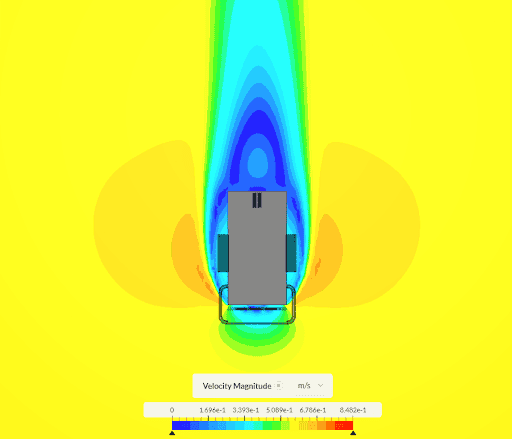
Eureka III descending
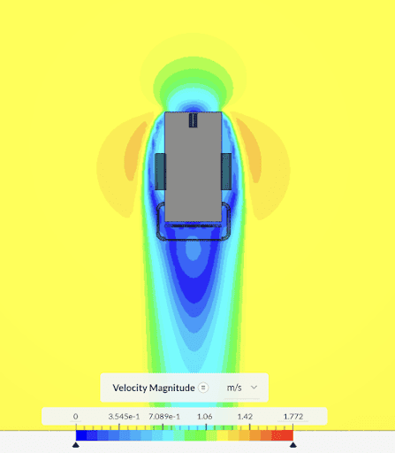
Eureka III ascending
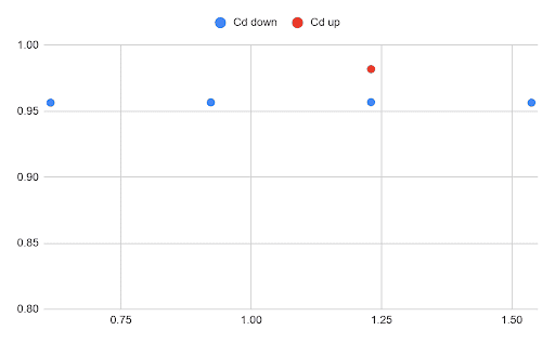
The chart below shows the calculated Cd for Eureka III vertical travel based on a series of CFD simulations conducted at different speeds and directions. There is a slightly higher Cd for ascending, compared to descending, and both have a Cd less than the assumed Cd in the TEA.
The other simplification that is built into the TEA for vertical travel is the travel profile. In our operations, the vehicle will enter the water negatively buoyant and reach a terminal velocity where the drag perfectly balances the gravity force. As the vehicle approaches the seafloor, water is pumped out of the tanks, making the vehicle naturally buoyant at the seafloor. On the ascent, water is pumped out, resulting in a similar acceleration profile as the deceleration profile on the descent. As the vehicle reaches the surface, the tanks are again partially flooded to achieve neutral buoyancy for recovery of the AUV below the wave-affected zone.
Some simplifying assumptions have been built into the TEA, so that precise estimation of the exact motion profile is not required while maintaining the accuracy of the overall travel time and thus economic accuracy in the model. In this simplified model used in the TEA we assume that:
- When pumping, the acceleration / deceleration results in an average velocity over that time equivalent to 67% of the terminal velocity.
- We assume that we have reached terminal velocity at the point when pumping is completed.
- We assume that we are immediately at terminal velocity at the surface for the full descent, rather than modelling an acceleration profile, and the same is true for the ascent, where we assume we are at terminal velocity until we stop and are in the recovery process.
To illustrate the comparison, a time-series simulation incorporating the velocity-dependent Cd derived from the CFD analysis was conducted to represent the actual motion profile, which is then evaluated against the assumed motion profile utilized in the TEA. Values from TEA 6.2, Eureka III are used for this comparison.
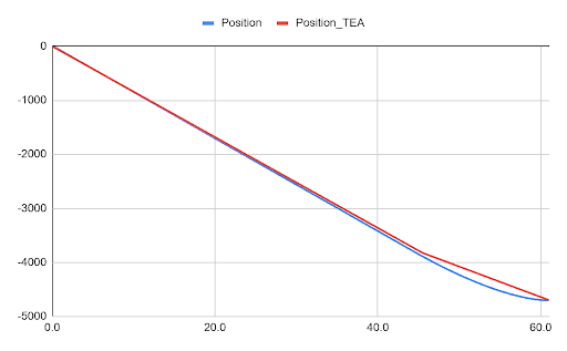
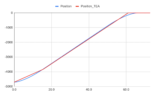
The combined time profiles using the simplified version in the TEA have a 2% difference for the amount of time the vehicles are in the water relative to the more involved motion profile determination. As one example of where the simplified analysis is a close approximation, in the more involved simulation, the AUV starts with a velocity of 0 and reaches the assumed TEA terminal velocity after only 25 seconds.
Both of these analyses assume that vertical travel is only controlled by the buoyancy engines. In reality, while the buoyancy engines will undoubtedly dominate the motion profiles, there is real potential for thrusters to be used during the pumping and valve phases to provide sharper acceleration and deceleration profiles, depending on what the overall system needs in terms of timing for any given vehicle.
Our techno-economic analysis (TEA) provides a powerful way to optimize design choices for our robotic collection system, even while relying on necessary simplifications to make the simulations efficient and valuable for iteration. By comparing assumed parameters, such as a fixed coefficient of drag and simplified motion profiles, against more detailed CFD simulations and time-series modeling, we’ve confirmed that the TEA remains an accurate tool for predicting performance. In fact, differences in predicted vertical travel time are on the order of only 2%, giving us confidence that the model captures the key dynamics while remaining practical for large-scale optimization.
